Using the USGS dataRetrieval package to analyze continuous water quality data

Last updated on Mar 14, 2023 R, Roadsalt, Water Quality

Introduction

As someone who works for the Division of Water Monitoring & Standards, I spend a lot of time analyzing water quality data. While we collect a significant amount of data in-house, I often need to download additional data from online sources. These sources typically come from the same organizations, and obtaining the necessary data requires navigating their websites, which can be a time-consuming process. However, I’m always on the lookout for ways to automate tasks and streamline my workflow. Recently, I discovered the dataRetrieval package, which provides a solution to this problem. With dataRetrieval, I can automate data retrieval tasks and avoid having to repeat the same steps over and over again.

What is the `dataRetrieval` package & how does it work?

The dataRetrieval package is a collection of functions designed to facilitate the retrieval of U.S. Geological Survey (USGS) and U.S. Environmental Protection Agency (EPA) water quality and hydrology data from web services. By using the dataRetrieval package, users can easily discover, access, retrieve, and parse water data from multiple sources. The data is obtained from various sources, and the image below provides a comprehensive overview of the different sources, data types, metadata, time series types, formats, and outputs available.

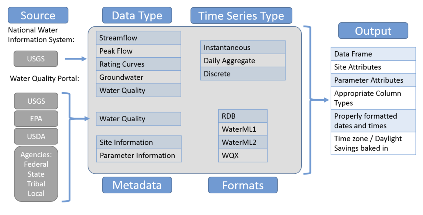
Image Credit: USGS

I’m not going to cover all the different functions and usages of the dataRetrieval package, but if you would like to learn more, here are some sources that I found to be the most useful:

What I will show in this blog post

In this blog post I will discuss the usage of the readNWISuv() function and how to create a nice plot with the ggplot2 package. The readNWISuv() function imports data from the NWIS web service. Specifically, this function retrieves instantaneous water quality data. In order to use this function you must have the following arguments:

readNWISuv(siteNumbers, parameterCd, startDate = "", endDate = "",tz = "UTC")

siteNumbers: A character vector of USGS site numbers (or multiple sites). This is usually an 8 digit number. You can use this map to find a site your interested in.
parameterCd: Character USGS parameter code.This is usually an 5 digit number. To find a parameter code of interest you can type in parameterCdFile. This allows you to explore the USGS parameter codes.
startDate: character starting date for data retrieval in the form YYYY-MM-DD.
endDate: character ending date for data retrieval in the form YYYY-MM-DD.
tz: character to set timezone attribute of dateTime. Default is “UTC”, and converts the date times to UTC. There are numerous different possible values to use. For example, if you wanted it to be in Eastern Standard Time, you would use "America/New_York"

Install and load `dataRetrieval` package from cran

   library(dataRetrieval)

Pull data with the `readNWISuv()` function

For my analysis, I am going to retrieve continuous specific conductance (SC) data for a site of interest in NJ using the dataRetrieval package. I will then use this specific conductance data to calculate Total Dissolved Solids (TDS) based on a correlation I established between SC and TDS. Since this isn’t the primary focus of this post, I won’t go into detail about the correlation. However, I plan to explain how I established it in a subsequent post.

USGS_continuous_sc_data<-readNWISuv("01408029","00095",tz = "America/New_York")

For simplicity, I am only looking up one site and one type of parameter. However, you can look up multiple sites and parameters in one pull. Now, let’s take a look at a preview of the data we just retrieved.

##   agency_cd  site_no            dateTime X_00095_00000 X_00095_00000_cd
## 1      USGS 01408029 2007-10-01 01:00:00           246                A
## 2      USGS 01408029 2007-10-01 01:15:00           246                A
## 3      USGS 01408029 2007-10-01 01:30:00           246                A
## 4      USGS 01408029 2007-10-01 01:45:00           246                A
## 5      USGS 01408029 2007-10-01 02:00:00           246                A
## 6      USGS 01408029 2007-10-01 02:15:00           246                A
##              tz_cd
## 1 America/New_York
## 2 America/New_York
## 3 America/New_York
## 4 America/New_York
## 5 America/New_York
## 6 America/New_York

The names of the columns in the dataframe can be described as follows:

agency_cd: The NWIS code for the agency reporting the data
site_no: The USGS site number
dateTime: The date and time of the value converted to UTC
X_00095_00000: The values of the parameter we gave to the function.
X_00095_00000_cd: The statistic code
tz_cd: The time zone code for dateTime

You can clean up the names with the reenameNWISColumns() function if you’d like.

We have the data… now what?

Now that we have retrieved the data, we can start manipulating it and creating a plot using the ggplot2 package. As mentioned earlier, I will calculate TDS because of a project related to roadsalt that I am working on. I wanted to include it in this post to demonstrate the wide range of options available in R. I will delve more into my roadsalt research in later posts!

What is the ggplot2 package?

The ggplot2 package is a system for ‘declaratively’ creating graphics, based on “The Grammar of Graphics”. It is a great way to visualize the data you are analyzing. With ggplot2, you have a lot of flexibility with the amount of customization you can give your plot. In my opinion, I think it is very easy to learn and it produces beautiful high quality plots. To learn more about ggplot2, I recommend The Complete ggplot2 Tutorial.

Full code used to create plot:

library(dataRetrieval)
library(ggplot2)
library(dplyr)
library(plyr)

### Vector of sites with continuous specific conductance data ###
siteNumber<-c("01408029")

### Parameter code for specific conductance ###
parameterCd<-"00095"

### Function that retrieves near real time continuous data for specific sites and parameters ###
USGS_continuous_sc_data<-readNWISuv(siteNumber,parameterCd,tz = "America/New_York")

### Filter dataframe ###
USGS_continuous_sc_data<-USGS_continuous_sc_data%>%
  dplyr::select(site_no,dateTime,X_00095_00000)%>%
  dplyr::rename(Site = site_no,Specific_conductance = X_00095_00000)
  
### Calculate TDS based on continuous Specific Conductance data and eq from correlation plots ###
final_USGS_data_TDS<-USGS_continuous_sc_data%>%
  dplyr::mutate(Calculated_TDS = Specific_conductance * 0.572 +6.19)

### theme for plots ###
graph_theme_T<- theme_linedraw()+
  theme(plot.title=element_text(size=15, face="bold",vjust=0.5,hjust = 0.5),
        plot.subtitle = element_text(size=15, face="bold",vjust=0.5,hjust = 0.5),
        panel.grid.major.x = element_blank(),
        panel.grid.minor.x = element_blank(),
        plot.background = element_blank(),
        panel.background = element_blank(),
        plot.margin = unit(c(1.5,2,4,2), "lines"), 
        legend.position = "bottom",
        legend.background = element_blank(),
        legend.text=element_text(size=10, face="bold"))
        
### Make plot of data ###
      
p<-ggplot(final_USGS_data_TDS, aes(x=dateTime,y=Calculated_TDS)) +
  geom_line(aes(color = "USGS Continuous Data"),
    stat = "identity",size=1.3)+
  scale_y_continuous(expand = c(0, 0), limits = c(0, max(final_USGS_data_TDS$Calculated_TDS)))+
  ggtitle("Total Dissolved Solids (TDS) Concentration (mg/L)") +
  labs(subtitle =paste("USGS Site:",final_USGS_data_TDS$Site,sep = ''))+
  xlab("Year") + ylab("TDS Concentration (mg/L)") +
  geom_hline(aes(yintercept = 500,color="Freshwater Aquatic Life Criteria for TDS = 500 mg/L"),size=1.3,alpha=0.6)+
  scale_color_manual("",
                     values = c("USGS Continuous Data"="#037907",
                                "Freshwater Aquatic Life Criteria for TDS = 500 mg/L"="red"))+
  
  graph_theme_T 

p

Final Product:

## Warning: Using `size` aesthetic for lines was deprecated in ggplot2 3.4.0.
## ℹ Please use `linewidth` instead.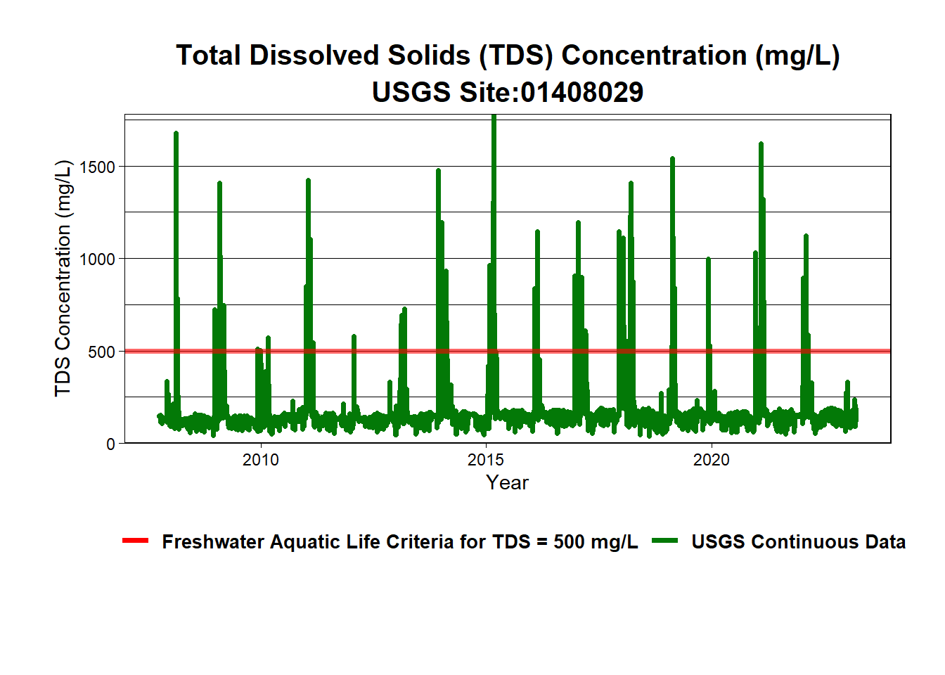

What is this plot showing?

This plot shows the calculated TDS concentration for the selected site from 2007 to the present day. The red line indicates the Freshwater Aquatic Life Criteria for TDS. In simplest terms, when the graph shows the TDS concentration (green line) going over the red line, TDS is above the standard.

Conclusion

The dataRetrieval package is an incredibly useful tool for water quality analysis. With just a few lines of code, you can obtain a vast amount of data. In this post, I have only covered one function, but there are many others available to access various types of water quality data. Be sure to review the resources I provided at the beginning of the post if you want to learn more. Although this post was basic, I hope it has been helpful in some way. If you have any questions, please do not hesitate to reach out to me!

R Water Quality Roadsalt

Using the USGS dataRetrieval package to analyze continuous water quality data

Introduction

What is the `dataRetrieval` package & how does it work?

What I will show in this blog post

Install and load `dataRetrieval` package from cran

Pull data with the `readNWISuv()` function

We have the data… now what?

What is the ggplot2 package?

Full code used to create plot:

Final Product:

What is this plot showing?

Conclusion

Kevin Zolea

Environmental Specialist

Using the USGS dataRetrieval package to analyze continuous water quality data

Introduction

What is the dataRetrieval package & how does it work?

What I will show in this blog post

Install and load dataRetrieval package from cran

Pull data with the readNWISuv() function

We have the data… now what?

What is the ggplot2 package?

Full code used to create plot:

Final Product:

What is this plot showing?

Conclusion

Kevin Zolea

Environmental Specialist

What is the `dataRetrieval` package & how does it work?

Install and load `dataRetrieval` package from cran

Pull data with the `readNWISuv()` function